Sparse Autoencoders can find interpretable features in Fourier Neural Operators

1. Background

1.1 Why an FNO?

A Fourier Neural Operator block does two things at every layer:

1. A spectral convolution: FFT the spatial input, multiply the low-frequency Fourier modes by a learned complex weight tensor, zero out (or ignore) the high modes, inverse-FFT back to spatial domain.
2. A local/pointwise path: usually a 1×1 convolution (or linear map) applied independently at each spatial location, added to the spectral path.
3. A nonlinearity (GELU/ReLU) applied to the sum.

That’s architecturally quite different from a transformer block, but it shares a property that matters for this experiment: at every spatial position, the network produces a fixed-width activation vector that is a genuine intermediate representation the model uses for computation. That means we can treat “one spatial position in one image” as a token, exactly the unit SAE work uses for token positions in a transformer’s residual stream. A 28×28 MNIST image passing through a block with 32 channels yields 784 tokens of dimension 32 — a lot of data from a small dataset.

1.2 Why an SAE?

The standard mechanistic-interpretability worry about raw activations is polysemanticity: a single neuron/channel often responds to several unrelated features because the model is packing more concepts into its activation space than it has dimensions (superposition). An SAE addresses this by learning an overcomplete, sparsely-activating dictionary:

x ∈ R^d               (raw activation, d = 32 here)
f = ReLU(W_enc x + b_enc)     ∈ R^h        (h = 8d = 256, overcomplete)
x_hat = W_dec f + b_dec       ∈ R^d        (reconstruction)

loss = ||x - x_hat||^2 + λ * ||f||_1

If the model really does represent more independent concepts than it has raw dimensions, an overcomplete, L1-regularized dictionary can in principle unpack them into (mostly) one-feature-per-concept directions, at the cost of each token activating only a handful of the h features. This is the same recipe used across most published transformer SAE work; the question here is purely whether it transfers to a convolutional/spectral vision model with no attention and no residual stream in the usual sense.

---

2. Methodology

2.1 Model and training

FNO2d classifier, trained on MNIST for 3 epochs, Adam optimizer, standard cross-entropy loss on the final pooled/classified output. Training converges very quickly:

epoch 0: train_loss=0.3143  test_acc=0.9857
epoch 1: train_loss=0.0411  test_acc=0.9896
epoch 2: train_loss=0.0222  test_acc=0.9911

A representative FNO block (illustrative structure matching the pipeline used):

class FNOBlock(nn.Module):
    def __init__(self, channels, modes1, modes2):
        super().__init__()
        self.spectral_conv = SpectralConv2d(channels, channels, modes1, modes2)
        self.local_conv = nn.Conv2d(channels, channels, kernel_size=1)
        self.act = nn.GELU()

    def forward(self, x):
        # x: (B, C, H, W)
        x_spec = self.spectral_conv(x)   # FFT -> mode-truncated linear mix -> iFFT
        x_local = self.local_conv(x)
        return self.act(x_spec + x_local)

2.2 Evolution of the model internals after successive blocks

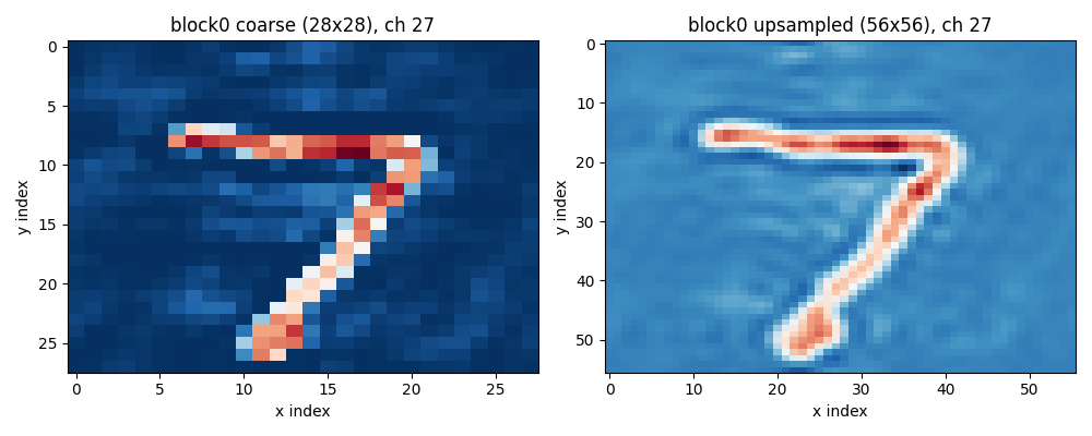
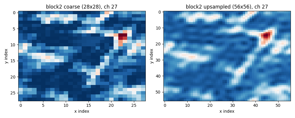
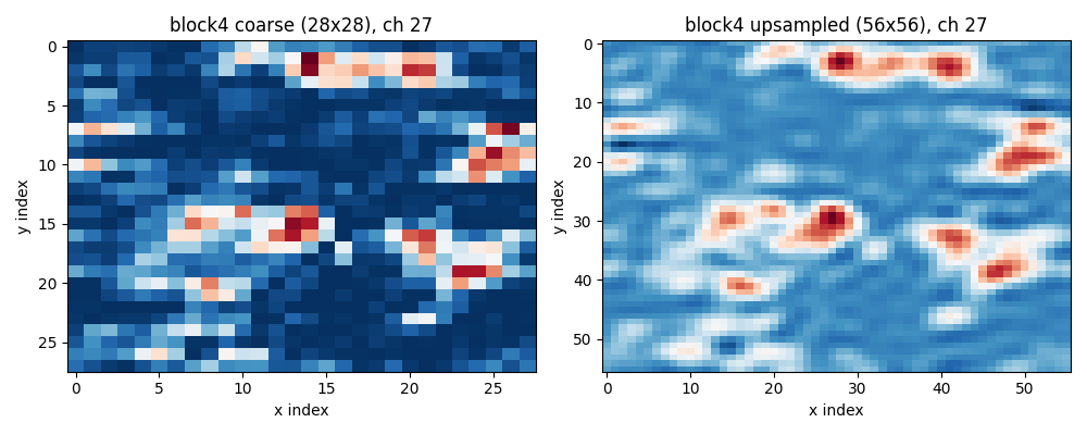
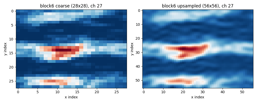
2.3 Hooking activations

Forward hooks are registered on each FNOBlock to capture its post-activation output before it’s overwritten by the next layer:

def register_block_hooks(model):
    activations = {}
    def make_hook(name):
        def hook(module, inp, out):
            activations[name] = out.detach()
        return hook
    handles = []
    for i, block in enumerate(model.blocks):
        handles.append(block.register_forward_hook(make_hook(f"block_{i}")))
    return activations, handles

Two blocks were probed across the reported runs: block 4 and block 6 (roughly mid-depth in the stack). Block 6 is the one carried through to the full analysis reported below.

2.4 Building the activation dataset

Each hooked activation tensor is (B, C, H, W). To train the SAE we flatten the spatial dimensions into the token axis, keeping the channel axis as the feature dimension:

@torch.no_grad()
def collect_block_activation_dataset(model, dataset, block_idx, n_images):
    activations, handles = register_block_hooks(model)
    loader = DataLoader(dataset, batch_size=256, shuffle=False)
    flat_chunks, raw_acts = [], []
    seen = 0
    for xb, _ in loader:
        model(xb.to(DEVICE))
        act = activations[f"block_{block_idx}"]        # (B, C, H, W)
        B, C, H, W = act.shape
        flat = act.permute(0, 2, 3, 1).reshape(-1, C)   # (B*H*W, C)
        flat_chunks.append(flat.cpu())
        raw_acts.extend([act[i].cpu() for i in range(B)])
        seen += B
        if seen >= n_images:
            break
    for h in handles:
        h.remove()
    return torch.cat(flat_chunks, dim=0), raw_acts, (H, W)

A label-carrying variant (collect_block_activation_dataset_with_labels) additionally returns the digit label alongside each token, used later for the class-selectivity analysis. Run at full scale over the test set this produces 7,840,000 tokens of dimension 32 — one 32-d vector per pixel per image, ~2000-7840 images depending on the run.

2.5 SAE architecture and training

class SAE(nn.Module):
    def __init__(self, d_in, d_hidden):
        super().__init__()
        self.W_enc = nn.Parameter(torch.randn(d_in, d_hidden) * 0.1)
        self.b_enc = nn.Parameter(torch.zeros(d_hidden))
        self.W_dec = nn.Parameter(torch.randn(d_hidden, d_in) * 0.1)
        self.b_dec = nn.Parameter(torch.zeros(d_in))
        self.register_buffer("feature_fire_count", torch.zeros(d_hidden))
        self.register_buffer("n_seen", torch.zeros(1))

    def encode(self, x):
        return F.relu((x - self.b_dec) @ self.W_enc + self.b_enc)

    def decode(self, f):
        return f @ self.W_dec + self.b_dec

    def forward(self, x):
        f = self.encode(x)
        x_hat = self.decode(f)
        return x_hat, f

def sae_loss(x, x_hat, f, l1_coeff):
    mse = F.mse_loss(x_hat, x)
    l1 = f.abs().sum(dim=-1).mean()
    return mse + l1_coeff * l1, mse.item(), l1.item()

Dictionary size d_hidden = 8 * d_in = 256 (8x overcomplete). Two l1_coeff settings were run: 1e-3 on unnormalized block-6/block-4 activations, and 1e-2 on normalized block-6 activations for the final analysis. Both trained for a small number of epochs (20 and 8 respectively) with Adam.

Representative training curve, final run (l1_coeff=1e-2, normalized):

SAE epoch 0: mse=0.84274  l1=43.50423
SAE epoch 1: mse=0.00368  l1=18.52292
SAE epoch 2: mse=0.01334  l1=18.66847
SAE epoch 3: mse=0.00725  l1=18.43291
SAE epoch 4: mse=0.00659  l1=18.04914
SAE epoch 5: mse=0.00566  l1=17.78640
SAE epoch 6: mse=0.00662  l1=17.66307
SAE epoch 7: mse=0.00620  l1=17.63719

Note the very sharp drop in MSE after epoch 0 (0.84 → 0.004) — the SAE essentially learns to reconstruct almost immediately, then spends the remaining epochs slowly trading a bit of reconstruction quality for sparsity as the L1 term pulls features toward zero.

2.6 Interpretability metrics

Three standard metrics, computed over a held-out slice of the activation dataset:

@torch.no_grad()
def interp_report(sae, flat_acts):
    x_hat, f = sae(flat_acts)
    resid_var = (flat_acts - x_hat).var()
    total_var = flat_acts.var()
    fvu = resid_var / total_var
    l0 = (f > 0).float().sum(dim=-1).mean()
    dead_frac = (sae.feature_fire_count == 0).float().mean()
    print(f"Fraction of variance unexplained: {fvu:.4f}  (explained: {1-fvu:.4f})")
    print(f"Mean L0 (active features / sample): {l0:.2f} / {f.shape[-1]}")
    print(f"Dead feature fraction: {dead_frac*100:.1f}%")

• Fraction of variance unexplained (FVU): how much reconstruction error remains, normalized by the variance of the original signal. Lower is better; 1 - FVU is the “variance explained” figure usually quoted.
• L0: average number of nonzero (post-ReLU) features per token. This is the direct measure of sparsity — the thing the L1 penalty is trying to minimize.
• Dead feature fraction: proportion of the 256 dictionary directions that never fire above zero across the evaluation set. A high dead fraction usually means the dictionary is oversized for the data, or that training collapsed onto too few directions.

2.7 Class-selectivity analysis

To check whether individual SAE features correspond to individual digit classes, we compute the mean activation of each feature conditioned on the ground-truth label, then rank features by an affinity score:

@torch.no_grad()
def compute_feature_selectivity(sae, flat_acts, flat_labels, scale, device, n_classes=10):
    x = (flat_acts * scale).to(device)
    f = sae.encode(x)                                  # (N, 256)
    class_means = torch.zeros(n_classes, f.shape[-1])
    for c in range(n_classes):
        mask = flat_labels == c
        class_means[c] = f[mask].mean(dim=0)

    results = []
    for feat_idx in range(f.shape[-1]):
        means = class_means[:, feat_idx]
        best_class = means.argmax().item()
        best_val = means[best_class].item()
        other_mean = (means.sum() - best_val) / (n_classes - 1)
        affinity = best_val - other_mean
        results.append({"feature_idx": feat_idx, "best_class": best_class, "affinity": affinity})
    results.sort(key=lambda r: -r["affinity"])
    return results

This is a deliberately simple metric — mean activation on the best class minus the mean over all other classes — and Section 4.2 discusses its main weakness.

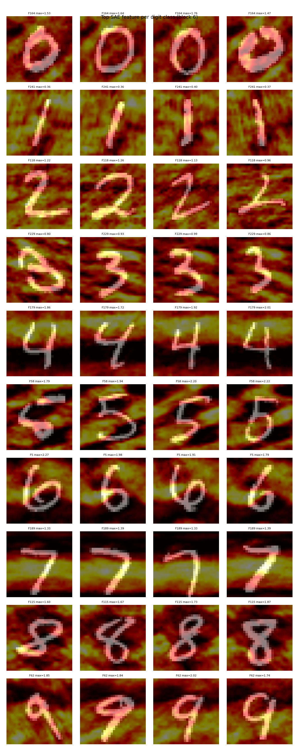
2.8 Spatial visualization

For a given SAE feature and a given raw (unflattened) activation map, we re-encode the map position-by-position and reshape the resulting per-position activation back into an (H, W) grid, which can then be overlaid on the source image:

@torch.no_grad()
def visualize_feature(sae, raw_acts, hw_shape, feature_idx, top_k=4):
    H, W = hw_shape
    scores = []
    for i, act in enumerate(raw_acts):
        C = act.shape[0]
        x = act.permute(1, 2, 0).reshape(-1, C).to(DEVICE)
        fmap = sae.encode(x)[:, feature_idx].reshape(H, W).cpu()
        scores.append((fmap.max().item(), i, fmap))
    scores.sort(key=lambda s: -s[0])
    top = scores[:top_k]
    # ... plotting: overlay fmap as a heat channel on top of the source digit image
    return top

3. Results

3.1 Class-selectivity table

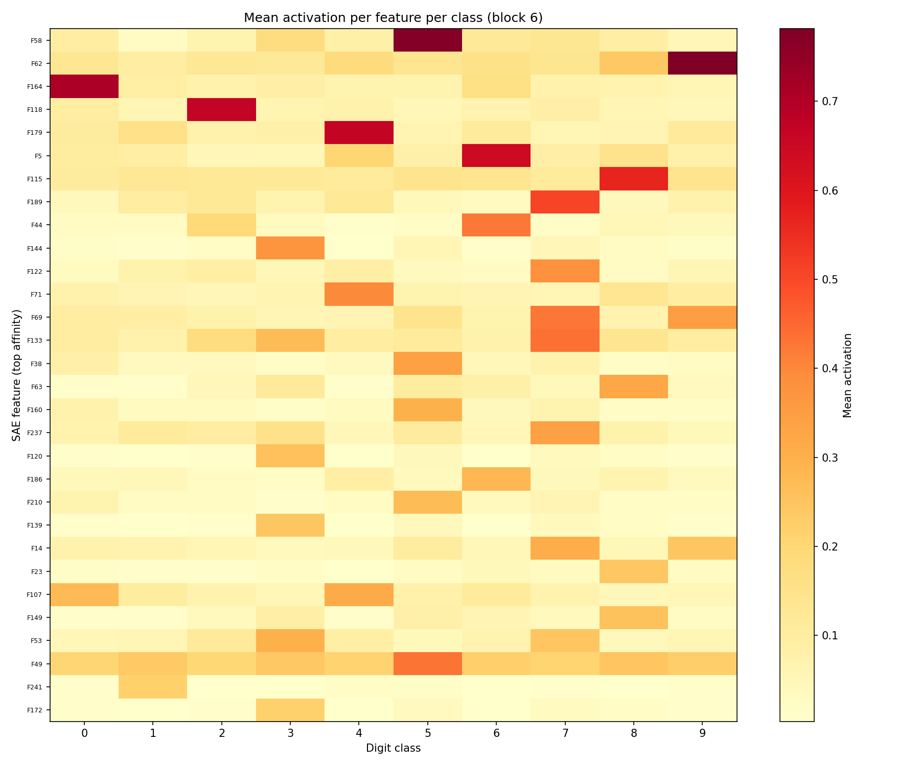
Top ten features by affinity (best-class mean minus mean over other classes), from the normalized block-6 run:

Feature	Best class	Affinity
58	5	0.6777
62	9	0.6355
164	0	0.6273
118	2	0.5968
179	4	0.5774
5	6	0.5434
115	8	0.4420
189	7	0.4372
44	6	0.3816
144	3	0.3469

The full 256-feature heatmap makes this pattern visible at scale — even outside the top 10, most rows show one or two clearly brighter cells rather than uniform low-level activation across all ten columns. Confusion matrix for all classes

3.2 Spatial coherence

Overlaying each top feature’s spatial activation map on real example digits addresses shows that for each number the sae has learned a different representation: